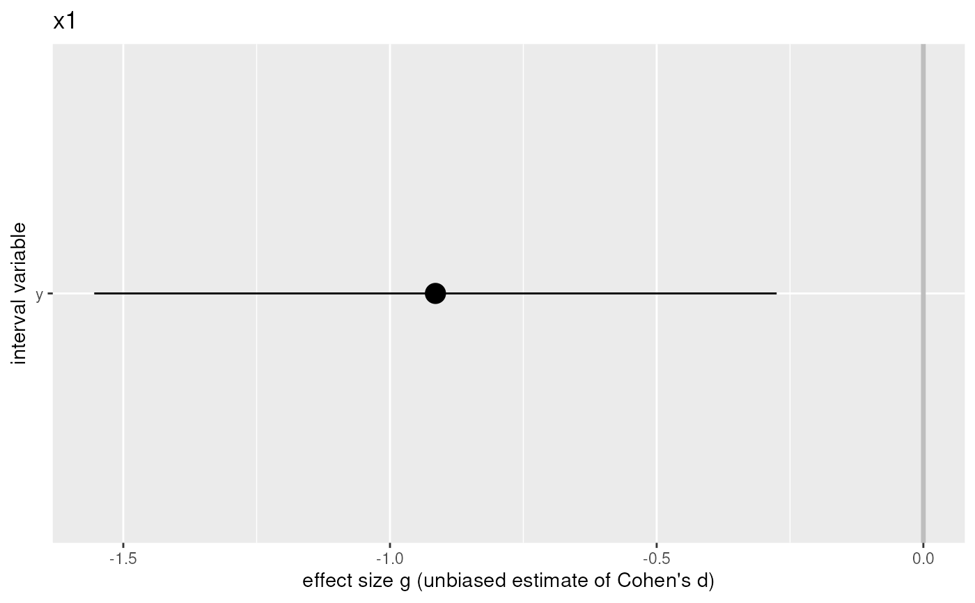
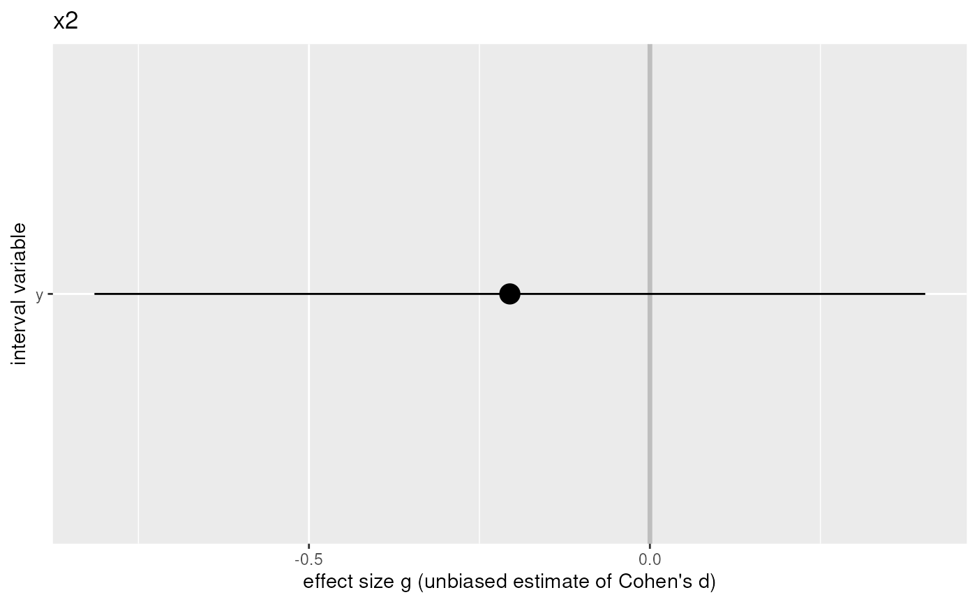
The meanDiff.multi function compares many means for many groups. It presents the results in a dataframe summarizing all relevant information, and produces plot showing the confidence intervals for the effect sizes for each predictor (i.e. dichotomous variable). Like meanDiff, it computes Cohen's d, the unbiased estimate of Cohen's d (Hedges' g), and performs a t-test. It also shows the achieved power, and, more usefully, the power to detect small, medium, and large effects.
meanDiff.multi(
  dat,
  y,
  x = NULL,
  var.equal = "yes",
  conf.level = 0.95,
  digits = 2,
  orientation = "vertical",
  zeroLineColor = "grey",
  zeroLineSize = 1.2,
  envir = parent.frame()
)

# S3 method for meanDiff.multi
print(x, digits = x$digits, powerDigits = x$digits + 2, ...)
Arguments
- dat
The dataframe containing the variables involved in the mean tests.
- y
Character vector containing the list of interval variables to include in the tests.
- x
Character vector containing the list of the dichotomous variables to include in the tests. If x is empty, paired samples t-tests will be conducted.
- var.equal
String; only relevant if x & y are independent; can be "test" (default; test whether x & y have different variances), "no" (assume x & y have different variances; see the Warning below!), or "yes" (assume x & y have the same variance)
- conf.level
Confidence of confidence intervals you want.
- digits
With what precision you want the results to print.
- orientation
Whether to plot the effect size confidence intervals vertically (like a forest plot, the default) or horizontally.
- zeroLineColor
Color of the horizontal line at an effect size of 0 (set to 'white' to not display the line; also adjust the size to 0 then).
- zeroLineSize
Size of the horizontal line at an effect size of 0 (set to 0 to not display the line; also adjust the color to 'white' then).
- envir
The environment where to search for the variables (useful when calling meanDiff from a function where the vectors are defined in that functions environment).
- powerDigits
With what precision you want the power to print.
- ...
Additional arguments are passed on to the
meanDiff()print methods.
Value
An object is returned with the following elements:
- results.raw
Objects returned by the calls to meanDiff.
- plots
For every comparison, a plot with the datapoints, means, and confidence intervals in the two groups.
- results.compiled
Dataframe with the most important results from each comparison.
- plots.compiled
For every dichotomous (x) variable, a plot with the confidence interval for the effect size of each dependent (y) variable.
- input
The arguments with which the function was called.
Details
This function uses the meanDiff function, which uses the formulae from Borenstein, Hedges, Higgins & Rothstein (2009) (pages 25-32).
Warning
Note that when different variances are assumed for the t-test (i.e. the null-hypothesis test), the values of Cohen's d are still based on the assumption that the variance is equal. In this case, the confidence interval might, for example, not contain zero even though the NHST has a non-significant p-value (the reverse can probably happen, too).
References
Borenstein, M., Hedges, L. V., Higgins, J. P., & Rothstein, H. R. (2011). Introduction to meta-analysis. John Wiley & Sons.
Examples
### Create simple dataset
dat <- data.frame(x1 = factor(rep(c(0,1), 20)),
                  x2 = factor(c(rep(0, 20), rep(1, 20))),
                  y=rep(c(4,5), 20) + rnorm(40));
### Compute mean difference and show it
meanDiff.multi(dat, x=c('x1', 'x2'), y='y', var.equal="yes");
#>    x y group1 group2    mean1    mean2       sd1      sd2 n1 n2          g
#> 1 x1 y      0      1 3.962437 4.764067 0.6776224 1.008105 20 20 -0.9147697
#> 2 x2 y      0      1 4.264056 4.462449 0.8670592 1.020371 20 20 -0.2053716
#>      g.ci.lo    g.ci.hi      pwr.g  pwr.small pwr.medium pwr.large          t
#> 1 -1.5544691 -0.2750704 0.82019177 0.09456733   0.337939 0.6934042 -2.9513928
#> 2 -0.8145175  0.4037743 0.09900971 0.09456733   0.337939 0.6934042 -0.6626065
#>   df           p
#> 1 38 0.005395123
#> 2 38 0.511581823
#> $x1

#>
#> $x2

#>
#> $x2
 #>
#>