This function is meant as a userfriendly wrapper to approximate the way analysis of variance is done in SPSS.
fanova(
  data,
  y,
  between = NULL,
  covar = NULL,
  withinReference = 1,
  betweenReference = NULL,
  withinNames = NULL,
  plot = FALSE,
  levene = FALSE,
  digits = 2,
  contrast = NULL
)

# S3 method for fanova
print(x, digits = x$input$digits, ...)
Arguments
- data
The dataset containing the variables to analyse.
- y
The dependent variable. For oneway anova, factorial anova, or ancova, this is the name of a variable in dataframe
data. For repeated measures anova, this is a vector with the names of all variable names in dataframedata, e.g.c('t0_value', 't1_value', 't2_value').- between
A vector with the variables name(s) of the between subjects factor(s).
- covar
A vector with the variables name(s) of the covariate(s).
- withinReference
Number of reference category (variable) for within subjects treatment contrast (dummy).
- betweenReference
Name of reference category for between subject factor in RM anova.
- withinNames
Names of within subjects categories (dependent variables).
- plot
Whether to produce a plot. Note that a plot is only produced for oneway and twoway anova and oneway repeated measures designs: if covariates or more than two between-subjects factors are specified, not plot is produced. For twoway anova designs, the second predictor is plotted as moderator (and the first predictor is plotted on the x axis).
- levene
Whether to show Levene's test for equality of variances (using
car'sleveneTestfunction but specifyingmeanas function to compute the center of each group).- digits
Number of digits (actually: decimals) to use when printing results. The p-value is printed with one extra digit.
- contrast
This functionality has been implemented for repeated measures only.
- x
The object to print (i.e. as produced by
regr).- ...
Any additional arguments are ignored.
Value
Mainly, this function prints its results, but it also returns them in an object containing three lists:
- input
The arguments specified when calling the function
- intermediate
Intermediat objects and values
- output
The results such as the plot.
Details
This wrapper uses oneway and lm and
lmer in combination with car's Anova
function to conduct the analysis of variance.
See also
Examples
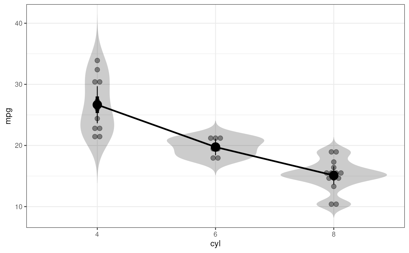
### Oneway anova with a plot
fanova(dat=mtcars, y='mpg', between='cyl', plot=TRUE);
#> Between-subjects factor cyl does not have class 'factor' in dataframe 'mtcars'. Converting it now.
#> Flexible Analysis of Variance was called with:
#>
#> Dependent variable: mpg
#> Factors: cyl
#>
#>
 #> Anova Table (Type III tests)
#>
#> Response: mpg
#> Sum Sq Df F value Pr(>F)
#> (Intercept) 7820.4 1 752.808 < 2.2e-16 ***
#> cyl 824.8 2 39.697 4.979e-09 ***
#> Residuals 301.3 29
#> ---
#> Signif. codes: 0 ‘***’ 0.001 ‘**’ 0.01 ‘*’ 0.05 ‘.’ 0.1 ‘ ’ 1
#>
#>
#> Partial omega squared effect sizes
#> value
#> 0.7074821
#>
#>
#> Parameter estimates, omnibus F-test and R-squared values
#>
#> Call:
#> stats::lm(formula = res$intermediate$formula, data = data, contrasts = contrastFunction)
#>
#> Residuals:
#> Min 1Q Median 3Q Max
#> -5.2636 -1.8357 0.0286 1.3893 7.2364
#>
#> Coefficients:
#> Estimate Std. Error t value Pr(>|t|)
#> (Intercept) 26.6636 0.9718 27.437 < 2e-16 ***
#> cyl6 -6.9208 1.5583 -4.441 0.000119 ***
#> cyl8 -11.5636 1.2986 -8.905 8.57e-10 ***
#> ---
#> Signif. codes: 0 ‘***’ 0.001 ‘**’ 0.01 ‘*’ 0.05 ‘.’ 0.1 ‘ ’ 1
#>
#> Residual standard error: 3.223 on 29 degrees of freedom
#> Multiple R-squared: 0.7325, Adjusted R-squared: 0.714
#> F-statistic: 39.7 on 2 and 29 DF, p-value: 4.979e-09
#>
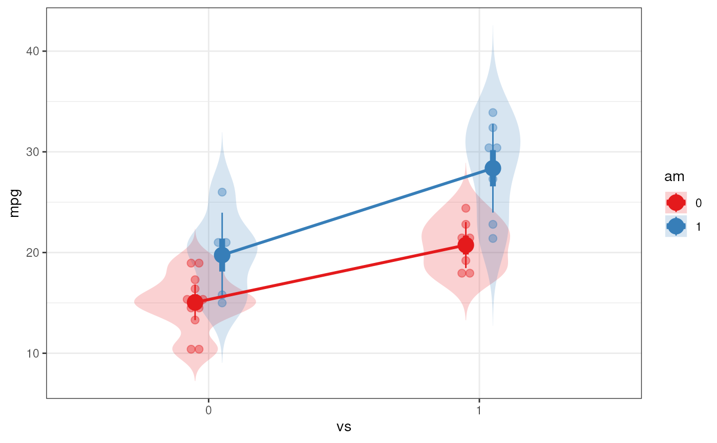
### Factorial anova
fanova(dat=mtcars, y='mpg', between=c('vs', 'am'), plot=TRUE);
#> Between-subjects factor vs does not have class 'factor' in dataframe 'mtcars'. Converting it now.
#> Between-subjects factor am does not have class 'factor' in dataframe 'mtcars'. Converting it now.
#> Flexible Analysis of Variance was called with:
#>
#> Dependent variable: mpg
#> Factors: vs & am
#>
#>
#> Anova Table (Type III tests)
#>
#> Response: mpg
#> Sum Sq Df F value Pr(>F)
#> (Intercept) 7820.4 1 752.808 < 2.2e-16 ***
#> cyl 824.8 2 39.697 4.979e-09 ***
#> Residuals 301.3 29
#> ---
#> Signif. codes: 0 ‘***’ 0.001 ‘**’ 0.01 ‘*’ 0.05 ‘.’ 0.1 ‘ ’ 1
#>
#>
#> Partial omega squared effect sizes
#> value
#> 0.7074821
#>
#>
#> Parameter estimates, omnibus F-test and R-squared values
#>
#> Call:
#> stats::lm(formula = res$intermediate$formula, data = data, contrasts = contrastFunction)
#>
#> Residuals:
#> Min 1Q Median 3Q Max
#> -5.2636 -1.8357 0.0286 1.3893 7.2364
#>
#> Coefficients:
#> Estimate Std. Error t value Pr(>|t|)
#> (Intercept) 26.6636 0.9718 27.437 < 2e-16 ***
#> cyl6 -6.9208 1.5583 -4.441 0.000119 ***
#> cyl8 -11.5636 1.2986 -8.905 8.57e-10 ***
#> ---
#> Signif. codes: 0 ‘***’ 0.001 ‘**’ 0.01 ‘*’ 0.05 ‘.’ 0.1 ‘ ’ 1
#>
#> Residual standard error: 3.223 on 29 degrees of freedom
#> Multiple R-squared: 0.7325, Adjusted R-squared: 0.714
#> F-statistic: 39.7 on 2 and 29 DF, p-value: 4.979e-09
#>
### Factorial anova
fanova(dat=mtcars, y='mpg', between=c('vs', 'am'), plot=TRUE);
#> Between-subjects factor vs does not have class 'factor' in dataframe 'mtcars'. Converting it now.
#> Between-subjects factor am does not have class 'factor' in dataframe 'mtcars'. Converting it now.
#> Flexible Analysis of Variance was called with:
#>
#> Dependent variable: mpg
#> Factors: vs & am
#>
#>
 #> Anova Table (Type III tests)
#>
#> Response: mpg
#> Sum Sq Df F value Pr(>F)
#> (Intercept) 2718.03 1 225.5116 6.344e-15 ***
#> vs 143.28 1 11.8878 0.001805 **
#> am 88.36 1 7.3311 0.011420 *
#> vs:am 16.01 1 1.3283 0.258855
#> Residuals 337.48 28
#> ---
#> Signif. codes: 0 ‘***’ 0.001 ‘**’ 0.01 ‘*’ 0.05 ‘.’ 0.1 ‘ ’ 1
#>
#>
#> Partial omega squared effect sizes
#> value
#> 0.6611129
#>
#>
#> Parameter estimates, omnibus F-test and R-squared values
#>
#> Call:
#> stats::lm(formula = res$intermediate$formula, data = data, contrasts = contrastFunction)
#>
#> Residuals:
#> Min 1Q Median 3Q Max
#> -6.971 -1.973 0.300 2.036 6.250
#>
#> Coefficients:
#> Estimate Std. Error t value Pr(>|t|)
#> (Intercept) 15.050 1.002 15.017 6.34e-15 ***
#> vs1 5.693 1.651 3.448 0.0018 **
#> am1 4.700 1.736 2.708 0.0114 *
#> vs1:am1 2.929 2.541 1.153 0.2589
#> ---
#> Signif. codes: 0 ‘***’ 0.001 ‘**’ 0.01 ‘*’ 0.05 ‘.’ 0.1 ‘ ’ 1
#>
#> Residual standard error: 3.472 on 28 degrees of freedom
#> Multiple R-squared: 0.7003, Adjusted R-squared: 0.6682
#> F-statistic: 21.81 on 3 and 28 DF, p-value: 1.735e-07
#>
### Ancova
fanova(dat=mtcars, y='mpg', between=c('vs', 'am'), covar='hp');
#> Between-subjects factor vs does not have class 'factor' in dataframe 'mtcars'. Converting it now.
#> Between-subjects factor am does not have class 'factor' in dataframe 'mtcars'. Converting it now.
#> Flexible Analysis of Variance was called with:
#>
#> Dependent variable: mpg
#> Factors: vs & am
#> Covariates: hp
#>
#>
#> Anova Table (Type III tests)
#>
#> Response: mpg
#> Sum Sq Df F value Pr(>F)
#> (Intercept) 865.64 1 113.1159 3.724e-11 ***
#> vs 7.56 1 0.9879 0.3290878
#> am 66.91 1 8.7437 0.0063831 **
#> hp 130.85 1 17.0993 0.0003093 ***
#> vs:am 12.26 1 1.6018 0.2164559
#> Residuals 206.62 27
#> ---
#> Signif. codes: 0 ‘***’ 0.001 ‘**’ 0.01 ‘*’ 0.05 ‘.’ 0.1 ‘ ’ 1
#>
#>
#> Partial omega squared effect sizes
#> value
#> 0.7839951
#>
#>
#> Parameter estimates, omnibus F-test and R-squared values
#>
#> Call:
#> stats::lm(formula = res$intermediate$formula, data = data, contrasts = contrastFunction)
#>
#> Residuals:
#> Min 1Q Median 3Q Max
#> -5.7169 -1.8183 0.5117 1.7778 4.8414
#>
#> Coefficients:
#> Estimate Std. Error t value Pr(>|t|)
#> (Intercept) 23.61868 2.22072 10.636 3.72e-11 ***
#> vs1 1.63180 1.64178 0.994 0.329088
#> am1 4.11159 1.39047 2.957 0.006383 **
#> hp -0.04413 0.01067 -4.135 0.000309 ***
#> vs1:am1 2.56502 2.02666 1.266 0.216456
#> ---
#> Signif. codes: 0 ‘***’ 0.001 ‘**’ 0.01 ‘*’ 0.05 ‘.’ 0.1 ‘ ’ 1
#>
#> Residual standard error: 2.766 on 27 degrees of freedom
#> Multiple R-squared: 0.8165, Adjusted R-squared: 0.7893
#> F-statistic: 30.04 on 4 and 27 DF, p-value: 1.377e-09
#>
### Don't run these examples to not take too much time during testing
### for CRAN
if (FALSE) {
### Repeated measures anova; first generate datafile
dat <- mtcars[, c('am', 'drat', 'wt')];
names(dat) <- c('factor', 't0_dependentVar' ,'t1_dependentVar');
dat$factor <- factor(dat$factor);
### Then do the repeated measures anova
fanova(dat, y=c('t0_dependentVar' ,'t1_dependentVar'),
between='factor', plot=TRUE);
}
#> Anova Table (Type III tests)
#>
#> Response: mpg
#> Sum Sq Df F value Pr(>F)
#> (Intercept) 2718.03 1 225.5116 6.344e-15 ***
#> vs 143.28 1 11.8878 0.001805 **
#> am 88.36 1 7.3311 0.011420 *
#> vs:am 16.01 1 1.3283 0.258855
#> Residuals 337.48 28
#> ---
#> Signif. codes: 0 ‘***’ 0.001 ‘**’ 0.01 ‘*’ 0.05 ‘.’ 0.1 ‘ ’ 1
#>
#>
#> Partial omega squared effect sizes
#> value
#> 0.6611129
#>
#>
#> Parameter estimates, omnibus F-test and R-squared values
#>
#> Call:
#> stats::lm(formula = res$intermediate$formula, data = data, contrasts = contrastFunction)
#>
#> Residuals:
#> Min 1Q Median 3Q Max
#> -6.971 -1.973 0.300 2.036 6.250
#>
#> Coefficients:
#> Estimate Std. Error t value Pr(>|t|)
#> (Intercept) 15.050 1.002 15.017 6.34e-15 ***
#> vs1 5.693 1.651 3.448 0.0018 **
#> am1 4.700 1.736 2.708 0.0114 *
#> vs1:am1 2.929 2.541 1.153 0.2589
#> ---
#> Signif. codes: 0 ‘***’ 0.001 ‘**’ 0.01 ‘*’ 0.05 ‘.’ 0.1 ‘ ’ 1
#>
#> Residual standard error: 3.472 on 28 degrees of freedom
#> Multiple R-squared: 0.7003, Adjusted R-squared: 0.6682
#> F-statistic: 21.81 on 3 and 28 DF, p-value: 1.735e-07
#>
### Ancova
fanova(dat=mtcars, y='mpg', between=c('vs', 'am'), covar='hp');
#> Between-subjects factor vs does not have class 'factor' in dataframe 'mtcars'. Converting it now.
#> Between-subjects factor am does not have class 'factor' in dataframe 'mtcars'. Converting it now.
#> Flexible Analysis of Variance was called with:
#>
#> Dependent variable: mpg
#> Factors: vs & am
#> Covariates: hp
#>
#>
#> Anova Table (Type III tests)
#>
#> Response: mpg
#> Sum Sq Df F value Pr(>F)
#> (Intercept) 865.64 1 113.1159 3.724e-11 ***
#> vs 7.56 1 0.9879 0.3290878
#> am 66.91 1 8.7437 0.0063831 **
#> hp 130.85 1 17.0993 0.0003093 ***
#> vs:am 12.26 1 1.6018 0.2164559
#> Residuals 206.62 27
#> ---
#> Signif. codes: 0 ‘***’ 0.001 ‘**’ 0.01 ‘*’ 0.05 ‘.’ 0.1 ‘ ’ 1
#>
#>
#> Partial omega squared effect sizes
#> value
#> 0.7839951
#>
#>
#> Parameter estimates, omnibus F-test and R-squared values
#>
#> Call:
#> stats::lm(formula = res$intermediate$formula, data = data, contrasts = contrastFunction)
#>
#> Residuals:
#> Min 1Q Median 3Q Max
#> -5.7169 -1.8183 0.5117 1.7778 4.8414
#>
#> Coefficients:
#> Estimate Std. Error t value Pr(>|t|)
#> (Intercept) 23.61868 2.22072 10.636 3.72e-11 ***
#> vs1 1.63180 1.64178 0.994 0.329088
#> am1 4.11159 1.39047 2.957 0.006383 **
#> hp -0.04413 0.01067 -4.135 0.000309 ***
#> vs1:am1 2.56502 2.02666 1.266 0.216456
#> ---
#> Signif. codes: 0 ‘***’ 0.001 ‘**’ 0.01 ‘*’ 0.05 ‘.’ 0.1 ‘ ’ 1
#>
#> Residual standard error: 2.766 on 27 degrees of freedom
#> Multiple R-squared: 0.8165, Adjusted R-squared: 0.7893
#> F-statistic: 30.04 on 4 and 27 DF, p-value: 1.377e-09
#>
### Don't run these examples to not take too much time during testing
### for CRAN
if (FALSE) {
### Repeated measures anova; first generate datafile
dat <- mtcars[, c('am', 'drat', 'wt')];
names(dat) <- c('factor', 't0_dependentVar' ,'t1_dependentVar');
dat$factor <- factor(dat$factor);
### Then do the repeated measures anova
fanova(dat, y=c('t0_dependentVar' ,'t1_dependentVar'),
between='factor', plot=TRUE);
}