This function is meant as a userfriendly wrapper to approximate the way logistic regression is done in SPSS.
logRegr(
  formula,
  data = NULL,
  conf.level = 0.95,
  digits = 2,
  predictGroupValue = NULL,
  comparisonGroupValue = NULL,
  pvalueDigits = 3,
  crossTabs = TRUE,
  oddsRatios = TRUE,
  plot = FALSE,
  collinearity = FALSE,
  env = parent.frame(),
  predictionColor = rosetta::opts$get("viridis3")[3],
  predictionAlpha = 0.5,
  predictionSize = 2,
  dataColor = rosetta::opts$get("viridis3")[1],
  dataAlpha = 0.33,
  dataSize = 2,
  observedMeansColor = rosetta::opts$get("viridis3")[2],
  binObservedMeans = 7,
  observedMeansSize = 2,
  observedMeansWidth = NULL,
  observedMeansAlpha = 0.5,
  theme = ggplot2::theme_bw(),
  headingLevel = 3
)

rosettaLogRegr_partial(
  x,
  digits = x$input$digits,
  pvalueDigits = x$input$pvalueDigits,
  headingLevel = x$input$headingLevel,
  echoPartial = FALSE,
  partialFile = NULL,
  quiet = TRUE,
  ...
)

# S3 method for rosettaLogRegr
knit_print(
  x,
  digits = x$input$digits,
  headingLevel = x$input$headingLevel,
  pvalueDigits = x$input$pvalueDigits,
  echoPartial = FALSE,
  partialFile = NULL,
  quiet = TRUE,
  ...
)

# S3 method for rosettaLogRegr
print(
  x,
  digits = x$input$digits,
  pvalueDigits = x$input$pvalueDigits,
  headingLevel = x$input$headingLevel,
  forceKnitrOutput = FALSE,
  ...
)
Arguments
- formula
The formula, specified in the same way as for
stats::glm()(which is used for the actual analysis).- data
Optionally, a dataset containing the variables in the formula (if not specified, the variables must exist in the environment specified in
env.- conf.level
The confidence level for the confidence intervals.
- digits
The number of digits used when printing the results.
- predictGroupValue, comparisonGroupValue
Can optionally be used to set the value to predict and the value to compare with.
- pvalueDigits
The number of digits used when printing the p-values.
- crossTabs
Whether to show cross tabulations of the correct predictions for the null model and the tested model, as well as the percentage of correct predictions.
- oddsRatios
Whether to also present the regression coefficients as odds ratios (i.e. simply after a call to
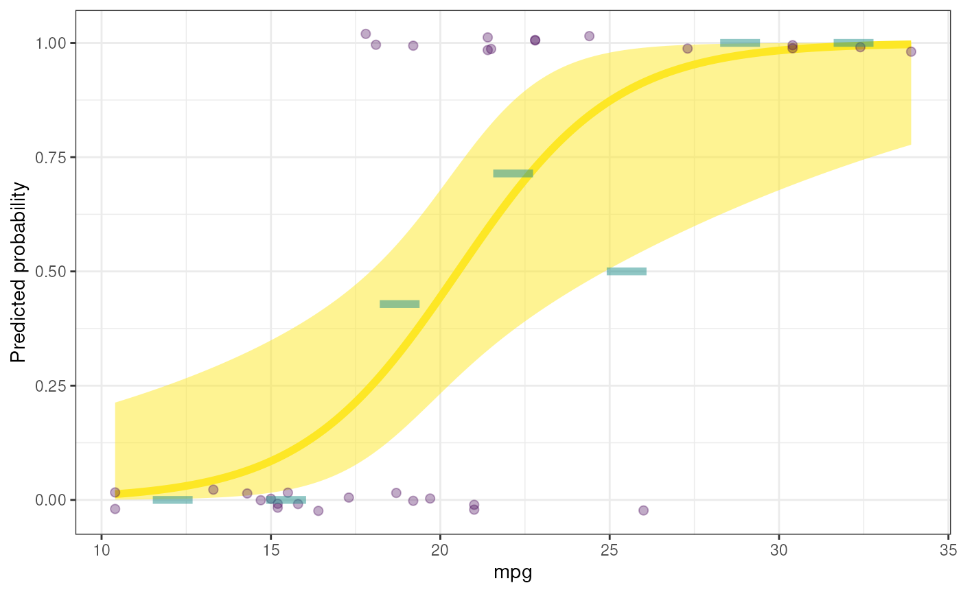
base::exp()).- plot
Whether to display the plot.
- collinearity
Whether to show collinearity diagnostics.
- env
If no dataframe is specified in
data, use this argument to specify the environment holding the variables in the formula.- predictionColor, dataColor, observedMeansColor
The color of, respectively, the line and confidence interval showing the prediction; the points representing the observed data points; and the means based on the observed data.
- predictionAlpha, dataAlpha, observedMeansAlpha
The alpha of, respectively, the confidence interval of the prediction; the points representing the observed data points; and the means based on the observed data (set to 0 to hide an element).
- predictionSize, dataSize, observedMeansSize
The size of, respectively, the line of the prediction; the points representing the observed data points; and the means based on the observed data (set to 0 to hide an element).
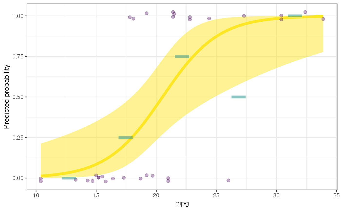
- binObservedMeans
Whether to bin the observed means; either FALSE or a single numeric value specifying the number of bins.
- observedMeansWidth
The width of the lines of the observed means. If not specified (i.e.
NULL), this is computed automatically and set to the length of the shortest interval between two successive points in the predictor data series (found usingufs::findShortestInterval().- theme
The theme used to display the plot.
- headingLevel
The number of hashes to print in front of the headings
- x
The object to print (i.e. as produced by
rosetta::logRegr).- echoPartial
Whether to show the executed code in the R Markdown partial (
TRUE) or not (FALSE).- partialFile
This can be used to specify a custom partial file. The file will have object
xavailable.- quiet
Passed on to
knitr::knit()whether it should b chatty (FALSE) or quiet (TRUE).- ...
Any additional arguments are passed to the default print method by the print method, and to
rmdpartials::partial()when knitting an RMarkdown partial.- forceKnitrOutput
Force knitr output.
Value
Mainly, this function prints its results, but it also returns them in an object containing three lists:
- input
The arguments specified when calling the function
- intermediate
Intermediat objects and values
- output
The results, such as the plot, the cross tables, and the coefficients.
See also
regr and fanova for similar functions
for linear regression and analysis of variance and stats::glm() for the
regular interface for logistic regression.
Examples
### Simplest way to call logRegr
rosetta::logRegr(data=mtcars, formula = vs ~ mpg);
#> Logistic regression analysis
#> Formula: vs ~ mpg
#> Sample size: 32
#> Predicting: 1
#>
#> Significance test of the entire model (all predictors together):
#> Cox & Snell R-squared: .44,
#> Nagelkerke R-squared: .58
#> Test for significance: ChiSq[1] = 18.33, p < .001
#>
#> Predictions by the null model (56.25% correct):
#>
#> Predicted
#> Observed 0
#> 0 18
#> 1 14
#>
#> Predictions by the tested model (81.25% correct):
#>
#> Predicted
#> Observed 0 1
#> 0 15 3
#> 1 3 11
#>
#> Raw regression coefficients (log odds values, called 'B' in SPSS):
#>
#> 95% conf. int. estimate se z p
#> (Intercept) [-16.74; -3.9] -8.83 3.16 -2.79 .005
#> mpg [0.18; 0.82] 0.43 0.16 2.72 .007
#>
#> Regression coefficients as odds ratios (ORs, called 'Exp(B)' in SPSS):
#>
#> OR 95% conf. int. OR point estimate
#> 1 [0; 0.02] 0.00
#> 2 [1.2; 2.28] 1.54
#>
### Also ordering a plot
rosetta::logRegr(
data=mtcars,
formula = vs ~ mpg,
plot=TRUE
);
#> Logistic regression analysis
#> Formula: vs ~ mpg
#> Sample size: 32
#> Predicting: 1
#>
#> Significance test of the entire model (all predictors together):
#> Cox & Snell R-squared: .44,
#> Nagelkerke R-squared: .58
#> Test for significance: ChiSq[1] = 18.33, p < .001
#>
#> Predictions by the null model (56.25% correct):
#>
#> Predicted
#> Observed 0
#> 0 18
#> 1 14
#>
#> Predictions by the tested model (81.25% correct):
#>
#> Predicted
#> Observed 0 1
#> 0 15 3
#> 1 3 11
#>
#> Raw regression coefficients (log odds values, called 'B' in SPSS):
#>
#> 95% conf. int. estimate se z p
#> (Intercept) [-16.74; -3.9] -8.83 3.16 -2.79 .005
#> mpg [0.18; 0.82] 0.43 0.16 2.72 .007
#>
#> Regression coefficients as odds ratios (ORs, called 'Exp(B)' in SPSS):
#>
#> OR 95% conf. int. OR point estimate
#> 1 [0; 0.02] 0.00
#> 2 [1.2; 2.28] 1.54
 #>
### Only use five bins
rosetta::logRegr(
data=mtcars,
formula = vs ~ mpg,
plot=TRUE,
binObservedMeans=5
);
#> Logistic regression analysis
#> Formula: vs ~ mpg
#> Sample size: 32
#> Predicting: 1
#>
#> Significance test of the entire model (all predictors together):
#> Cox & Snell R-squared: .44,
#> Nagelkerke R-squared: .58
#> Test for significance: ChiSq[1] = 18.33, p < .001
#>
#> Predictions by the null model (56.25% correct):
#>
#> Predicted
#> Observed 0
#> 0 18
#> 1 14
#>
#> Predictions by the tested model (81.25% correct):
#>
#> Predicted
#> Observed 0 1
#> 0 15 3
#> 1 3 11
#>
#> Raw regression coefficients (log odds values, called 'B' in SPSS):
#>
#> 95% conf. int. estimate se z p
#> (Intercept) [-16.74; -3.9] -8.83 3.16 -2.79 .005
#> mpg [0.18; 0.82] 0.43 0.16 2.72 .007
#>
#> Regression coefficients as odds ratios (ORs, called 'Exp(B)' in SPSS):
#>
#> OR 95% conf. int. OR point estimate
#> 1 [0; 0.02] 0.00
#> 2 [1.2; 2.28] 1.54
#>
### Only use five bins
rosetta::logRegr(
data=mtcars,
formula = vs ~ mpg,
plot=TRUE,
binObservedMeans=5
);
#> Logistic regression analysis
#> Formula: vs ~ mpg
#> Sample size: 32
#> Predicting: 1
#>
#> Significance test of the entire model (all predictors together):
#> Cox & Snell R-squared: .44,
#> Nagelkerke R-squared: .58
#> Test for significance: ChiSq[1] = 18.33, p < .001
#>
#> Predictions by the null model (56.25% correct):
#>
#> Predicted
#> Observed 0
#> 0 18
#> 1 14
#>
#> Predictions by the tested model (81.25% correct):
#>
#> Predicted
#> Observed 0 1
#> 0 15 3
#> 1 3 11
#>
#> Raw regression coefficients (log odds values, called 'B' in SPSS):
#>
#> 95% conf. int. estimate se z p
#> (Intercept) [-16.74; -3.9] -8.83 3.16 -2.79 .005
#> mpg [0.18; 0.82] 0.43 0.16 2.72 .007
#>
#> Regression coefficients as odds ratios (ORs, called 'Exp(B)' in SPSS):
#>
#> OR 95% conf. int. OR point estimate
#> 1 [0; 0.02] 0.00
#> 2 [1.2; 2.28] 1.54
 #>
if (FALSE) {
### Mimic output that would be obtained
### when calling from an R Markdown file
rosetta::rosettaLogRegr_partial(
rosetta::logRegr(
data=mtcars,
formula = vs ~ mpg,
plot=TRUE
)
);
}